Need to compute the square root of a number? Forget the calculator; use a ball, a stopwatch, and a vacuum chamber. Actually… yeah, maybe a calculator may be faster.

Computers are fast, and every day we try to make them faster. In terms of clock speed, however, they seem to be plateauing at 6 GHz. Additionally, as we shrink lithography processes, we are approaching a limit at which logic gates no longer behave as expected. In turn, people have been looking at quantum computers, but they are not miniaturizations of modern chips. Instead, quantum computing is a massive comeback of analog computing; it harnesses continuous waves for sophisticated calculations.

This article first explores concepts of analog computing, relevant quantum definitions, and an example to illustrate how quantum computing differs. The goal is to introduce the subject in a fresh way and set the stage for more hands-on experiments and mathematical details in future articles. With this context established, let us start by analyzing quantum computers.

Analog Computing

Analog computing is very powerful. Although digital computers dominate today, there are scenarios where analog systems may perform better. For example, NASA’s Automaton Rover for Extreme Environments (AREE) “replaces vulnerable electronics with an entirely mechanical design” ^[1]. In extreme environments, analog approaches may prove more stable. With this idea in mind, let’s explore some detailed cases of analog computing.

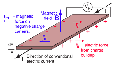
Multiplication with the Hall Effect

Let’s start with computing multiplications with electricity, not logic gates. Yes, it is possible to multiply two numbers using a current (the multiplicand) and a magnetic field (the multiplier), producing the result as the output voltage.

Figure 1. Properties of a conductive plate, and the setup to compute a multiplication. Source: ^[2].

⚠️ JavaScript is disabled. Mathematical formulas cannot be rendered.

The formula is simple:

$$ V_{out} = \frac{IB}{ned} = IBk $$

where $\frac{1}{ned}$ can be reduced to a constant $k$ based on the material used for the plate:

• $n$ is the number of charge carriers per unit volume.
• $e$ is the charge of an electron ($1.602 \times 10^{-19} C$).
• $d$ is the thickness of the conductor.

Gravity to Compute Square Roots

⚠️ JavaScript is disabled. Mathematical formulas cannot be rendered.

Interestingly, we don’t have to rely on electricity, and the computations can be more complex. Another fantastic example, as in the introduction to this article, is using gravity to compute square roots. Recall, from physics, the vertical position formula of an object:

$$ y(t) = y_{0y} + v_{0y} t - \frac{1}{2}gt^2 $$

Assume there is no initial velocity, position the origin at the object, and invert the y-axis so that the positive values go down (we are basically measuring the distance traveled).

$$ d = \frac{1}{2}gt^2 $$

Let’s solve for time.

$$ t = \sqrt{\frac{2d}{g}} $$

We must drop the object from a distance $d = \frac{gn}{2}$.

Let’s compute the square root of 100.

• $g = 9.81\ m/s^2$
• $n = 100$
• $d = 490.5\ m$

The result? The object will touch the floor in $\sqrt{\frac{2 \cdot 490 \cdot 5}{9.81}} = 10\ s$.

Figure 2. Example of computing the square root of a number using a ball and gravity. Source: ^[3].

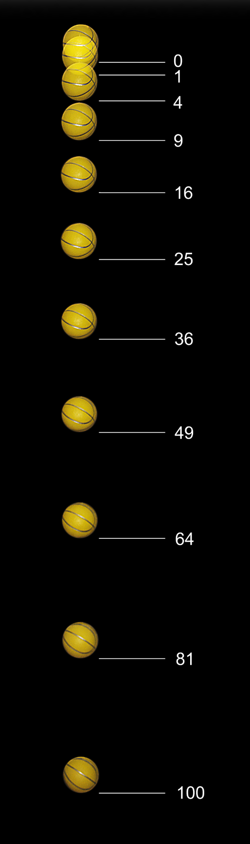
Oh, and don’t forget to perform this experiment in a vacuum chamber since we are not accounting for friction.

While this gravity-based example may not outpace a CPU—especially as values get larger—it offers other benefits. Like NASA’s AREE, such analog methods resist radiation (if you also use an analog stopwatch, of course). Now that we’ve seen analog computing’s approach, let’s consider computation using quantum properties.

Many Possibilities

It is possible to compute with many other things, such as pipes, steam, gears, springs, water, and DNA. Why bother with quantum? Each tool has its strengths and weaknesses. Quantum computers are better for problems that can be modeled in terms of interference. ^[4]

To set up an experiment using quantum mechanics for computation, it’s important to first define key properties and concepts.

Quantum Computing Concepts

Figure 3. Illustration of the definitions described in this article; generated by Google Gemini, 3 February 2026.

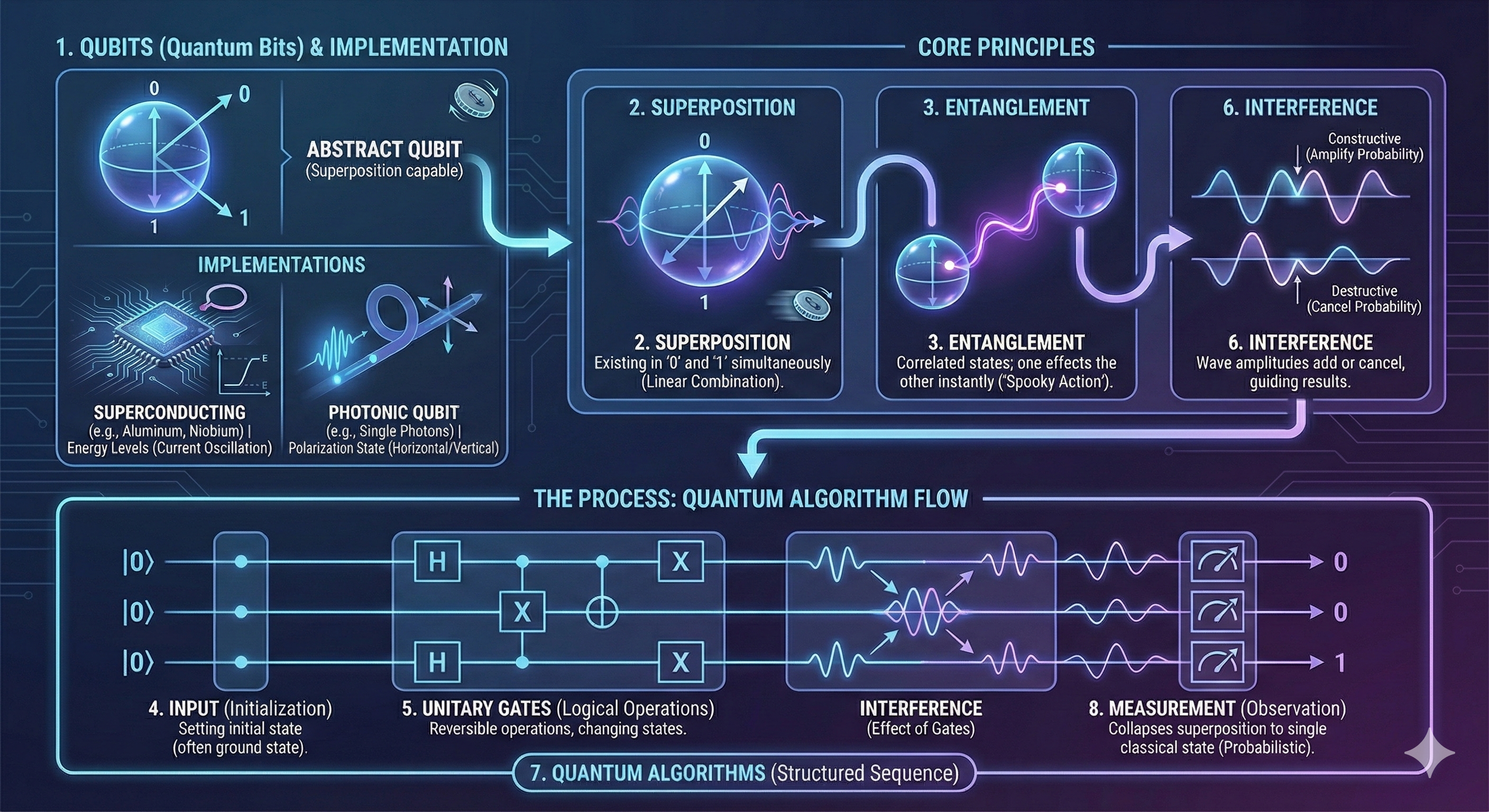
Qubits

Multiple sources compare classical bits used by traditional computers (1s and 0s) with qubits used by quantum computers, as in ^[5], ^[6], and ^[7]. Qubits are, in fact, the basic unit of information in quantum computers. They are usually encoded in the physical properties of particles (e.g., spin or polarization), just as classical bits are encoded in voltage states through circuits. However, they operate very differently; while a classical bit can have values of 1 or 0, a qubit usually can take the values 0, 1, or a complex combination of both ^[5].

How are qubits usually encoded into the physical properties of particles? It may be difficult to imagine coming from a classical computing background. It may help to understand the materials used to encode qubits. Here are two examples:

• Superconducting Qubits (Transmons): These are made of superconducting materials, such as aluminum, at extremely low temperatures. Then, the qubit states are represented by the energy levels: “the ground state (0)[, the] excited state (1)[, and using microwaves, the] transition between these two” ^[8].
• Photonic Qubits: These are made of single particles of light (photons) moving through waveguide or fiber. The qubit state is represented by the polarization of the light ^[9].

However, other implementations use trapped ions, quantum dots, topological systems, and more ^[10].

The two examples above briefly explain how the combination of both states 0 and 1 is achieved. That property has a name: superposition.

Superposition

⚠️ JavaScript is disabled. Mathematical formulas cannot be rendered.

Superposition is the property that qubits can be in a state that represents a linear combination of both $|0\rangle$ and $|1\rangle$.

An intuitive way to look at it is as “a bucket of red and blue marbles. Until you draw a marble, the outcome is characterized as $\frac{r}{r+b}$ red + $\frac{b}{r+b}$ blue. Once you draw from the bucket, that outcome has collapsed to either fully red or fully blue. Moreover, if you look at that drawn marble any number of times, it stays the same color” ^[3].

A later article on reversible computing will cover an experiment (the double-slit experiment) that demonstrates the difference between superposition and collapsed states.

Entanglement

Entanglement is a fascinating property of qubits. When two qubits become entangled, their states are correlated. In other words, “[w]e can entangle two quantum bits so that they randomly both measure either True or False, even if they are separated by light years from each other” ^[3].

Decoherence

Decoherence is the process that causes qubits to lose their quantum behavior (superposition and entanglement) and collapse into a nonquantum state, a classical bit (either 1 or 0). “It can be intentionally triggered by measuring a quantum system or by other environmental factors[.] Generally[, the standard practice involves] avoiding and minimizing decoherence” ^[5]. In other words, once decoherence happens, the qubit behaves like a particle that can only be in an absolute state of 1 or 0, but not the superposition of both.

Input

In classical computers, we usually set the inputs of a circuit (or program) by manipulating the voltages on the input pins. In quantum computers, we must first change the state of quantum particles so they behave like waves (in a superposition state) ^[11]. The previous definitions of qubits briefly touch on how to set the particles into the quantum state, which varies depending on the implementation. For example, if it is a transmon, the process may involve extreme cooling and firing a laser; if it is a photon, it is just a matter of firing a new photon.

⚠️ JavaScript is disabled. Mathematical formulas cannot be rendered.

Regardless, starting a new quantum program means starting with qubits in the ground state (that is, $|0\rangle$). Just like with classical circuits, one must change those inputs into a set that encodes the problem. In other words, the first step in a quantum program will be to set the qubits to the desired quantum state.

(Unitary) Gate

Once the particles are in a quantum state, the next step is about applying the desired logic. In quantum computing, that means using unitary quantum gates. Those are the ones responsible for changing the qubit states or creating complex superpositions.

They are unitary because they “are represented by unitary matrices, meaning they preserve the total probability of all possible outcomes (i.e., no information is lost during their operation)” ^[12]. These gates must be unitary because they must be reversible; however, that is a topic the next article may address.

Interference

Figure 4. Image illustrating wave interference. Source: ^[13]

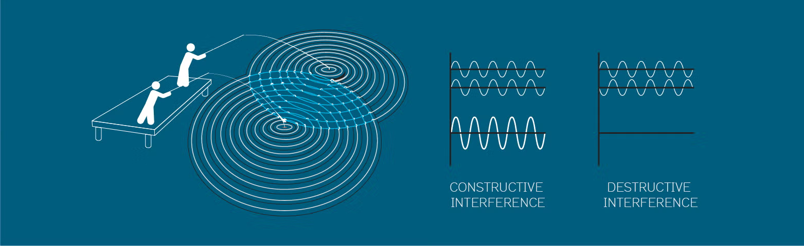
As the different input qubits interact with quantum gates, they start creating complex superpositions and entangle with each other. The power of quantum computers lies in the interaction between different particles. That interaction happens thanks to the interference.

Interference is like how waves interact with each other. There will be times when the interaction between two waves adds (constructive interference), and there will be times when they subtract (destructive interference). Fig. 4 shows an example of how interference works in waves; however, it is important to note that the “waves” representing the probabilities in qubits must always sum to 100%. Another crucial aspect is that the goal of quantum computing is to “amplify the probability of correct outcomes and suppress incorrect ones” ^[14].

Quantum Algorithms

Simply put, quantum algorithms are sequences of gates (or operations) that solve problems, just as classical computers do. In a way, it is about harnessing the properties of quantum mechanics (superpositions, entanglement, interference) to our advantage to solve problems that lend themselves better to interference.

Measurement

Measurement is different for quantum computers; it must happen at the end (unless you are working with measurement-based quantum computers, but that is a topic for another time). Otherwise, measuring a qubit in the middle of an operation causes it to lose its quantum behavior (see decoherence).

Limitations

This section introduced the main concepts relevant to quantum computing. Yes, it is crucial for future articles on this topic, but before we get into this section, we discussed other types of analog computing. Recall, a highlight was that different analog devices have different strengths and weaknesses. Quantum computing is no different.

The reader may be able to discern that quantum computers are well-suited for modeling some problems (just as gravity is well-suited for calculating square roots), but other problems may be better suited to other computing systems. For example, do you want to multiply a list of numbers? A traditional computer or calculator will suffice. Using a quantum computer for that is extremely expensive, and it may require a complicated series of quantum gates; classical computers nowadays have native commands that can handle that task flawlessly (oh, modern quantum computers also have an inherent error rate).

Let us finish by observing an experiment. That may help understand the power of quantum computers and why they require complex numbers rather than classical probabilities.

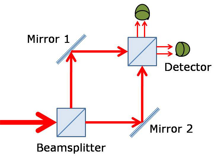
The Mach-Zehnder Interferometer

⚠️ JavaScript is disabled. Mathematical formulas cannot be rendered.

When discussing superposition, quantum particles were described as marbles. Before you draw the marble, there is a probability that you will get $\frac{r}{r+b}$ red or $\frac{b}{r+b}$ blue marbles. Qubits can represent more complex states than just probabilities. The Mach-Zehnder Interferometer experiment may help understand that concept.

Let us discuss the setup first (see Fig. 5). The experiment is about detecting the different paths a beam of light (or a photon) can take. First, fire the light towards a beamsplitter that has a 50% chance of letting light through and 50% chance of reflecting it. Then, there are two mirrors so that the two paths the light takes meet in a new beamsplitter. Then again, the beam splitter presents the light with two paths it can take, each with a detector at the end.

Figure 5. Illustration of the Mach-Zehnder interferometer experiment. Source: ^[15]

Particle Intuition

Consider the light a photon particle. The particle must take one of the two paths at the first beamsplitter, leading it to the upper or lower path.

⚠️ JavaScript is disabled. Mathematical formulas cannot be rendered.

• Probability of the particle taking the upper path: $P(U) = 1/2 = 50%$.
• Probability of the particle taking the lower path: $P(L) = 1/2 = 50%$.

Then, the second beamsplitter presents each path with the same choices:

⚠️ JavaScript is disabled. Mathematical formulas cannot be rendered.

• Probability that if the particle takes the upper path, P(U), it will be reflected, P(R), ending in the upper detector: $P(U) \cdot P(R) = \frac{1}{2} \cdot \frac{1}{2} = 25%$.
• Probability that if the particle takes the upper path, P(U), it will be transmitted, P(T), ending in the side detector: $P(U) \cdot P(T) = \frac{1}{2} \cdot \frac{1}{2} = 25%$.
• Probability that if the particle takes the lower path, P(L), it will be reflected, P(R), ending in the side detector: $P(L) \cdot P(R) = \frac{1}{2} \cdot \frac{1}{2} = 25%$.
• Probability that if the particle takes the lower path, P(L), it will be transmitted, P(T), ending in the upper detector: $P(L) \cdot P(T) = \frac{1}{2} \cdot \frac{1}{2} = 25%$.

Finally, add those results to get the probabilities that the particle will end in the upper or side detector.

⚠️ JavaScript is disabled. Mathematical formulas cannot be rendered.

• $P(Side Detector) = P(U) \cdot P(T) + P(L) \cdot P(R) = 50%$
• $P(Upper Detector) = P(L) \cdot P(T) + P(U) \cdot P(R) = 50%$

Well, that does not happen.

Real Quantum Behavior

Figure 5. Screenshot of the Mach-Zehnder interferometer setup in the Quantum Flytrap virtual lab.

Fig. 6 shows the actual result of the Mach-Zehnder interferometer experiment. The photon particle will always be detected by one of the detectors.

⚠️ JavaScript is disabled. Mathematical formulas cannot be rendered.

The reason is that we are omitting the wave phase, interference, superposition, and everything defined earlier. Every time the wave gets reflected, its phase shifts by 90° (or $\frac{\pi}{2}$). The upper detector will have two waves that have a phase shift of 180° (or $\pi$); in other words, they will cancel each other (recall the concept of destructive interference). On the other hand, the two waves that meet at the side detector are in phase, reinforcing the amplitude of the correct answer (constructive interference).

Mathematically, this process requires the use of complex numbers to capture the phase of the waves. A phase shift of 90° is a multiplication by $i = \sqrt{-1}$. Additionally, every time the light path is split in the beamsplitter, its amplitude splits into $\frac{1}{\sqrt{2}}$ (that is, the square root of the probability $\frac{1}{2}$ for each path). A later article may explain why; for now, accept these as definitions.

Recall that the set of complex numbers is: $\mathbb{C} = \{a + bi\ |\ a,b∈\mathbb{R}\wedge i=\sqrt{-1}\}$.

Let’s try the computation again with this new information!

The Mathematical Computation

The paths that lead to the side detector:

⚠️ JavaScript is disabled. Mathematical formulas cannot be rendered.

• Upper Path:
  • Reflects at the first beamsplitter, which shifts the phase ($i$) and changes the amplitude $\left( \frac{1}{\sqrt{2}} \right)$.
  • Reflects in the mirror, which only affects the phase again ($i$).
  • Transmits through the second beamsplitter, which changes the amplitude again (to $\frac{1}{\sqrt{2}}$ of its input).
  $$ Amplitude = \frac{i}{\sqrt{2}} \cdot i \cdot \frac{1}{\sqrt{2}} = \frac{i^2}{2} = - \frac{1}{2} $$
• Lower Path:
  • Transmits through the first beamsplitter, which only changes the amplitude $\left( \frac{1}{\sqrt{2}} \right)$.
  • Reflects in the mirror, which only affects the phase ($i$).
  • Reflects through the second beamsplitter, which changes the amplitude (to $\frac{1}{\sqrt{2}}$ of its input) and phase ($i$) again.
  $$ Amplitude = \frac{1}{\sqrt{2}} \cdot i \cdot \frac{i}{\sqrt{2}} = \frac{1}{2} = - \frac{1}{2} $$

Add both amplitudes:

$$ - \frac{1}{2} + \left( - \frac{1}{2} \right) = -1 $$

That is the square root of the probability. Squaring the magnitude produces the final probability:

$$ P(Side Detector) = |-1|^2 = 1 = 100% $$

Try computing the probability for the other detector using the same logic. It should produce a result that looks like this:

$$ P(Upper Detector) = |\left( \frac{i}{\sqrt{2}} \cdot i \cdot \frac{i}{\sqrt{2}} \right) + \left( \frac{1}{\sqrt{2}} \cdot i \cdot \frac{1}{\sqrt{2}} \right)|^2 = |\frac{i^3}{2}+\frac{i}{2}|^2 = |- \frac{i}{2} + \frac{i}{2}|^2 = 0% $$

These are all probabilities in a superposition. You haven’t drawn the marble (even though the analogy isn’t accurate). In other words, you still must measure the results. That is what the detectors do at the end of the circuit.

The side detector will receive all the light, while the upper detector receives nothing. It is crucial to measure the photon at the end, since that collapses its quantum state into a classical 0 or 1. In this case, the side detector measures 1, while the upper detector measures 0.

Conclusion

Hopefully, this exploration highlighted that quantum computers are not a matter of miniaturization or a breakthrough in how to make a processor run at 100 GHz. Instead, the innovation of quantum computers is taking us from working in an abstract logical domain (the digital computers) to harnessing natural laws (quantum mechanics). In other words, it moves computations from binary logic to continuous physics. Recall the Mach-Zehnder interferometer; it did not calculate the result using logic gates, but the result was the consequence of waves canceling the wrong answer.

However, just like classical physics has laws, so does quantum mechanics. Those rules lead us to an important concept to keep in mind when programming quantum computing (and the topic of the next article): reversible computations.

References

1. J. Sauder, “National Aeronautics and Space Administration,” 7 April 2016. [Online]. Available: https://www.nasa.gov/general/automaton-rover-for-extreme-environments-aree-2/. [Accessed 1 February 2026].
2. R. Nave, “Hall Effect,” 2019. [Online]. Available: http://hyperphysics.phy-astr.gsu.edu/hbase/magnetic/Hall.html. [Accessed 1 February 2026].
3. Z. Yang, “Introduction,” lecture slides for COT 5930: Introduction to Quantum Computing, COECS, Florida Atlantic University, Boca Raton, FL, United States, 14 January 2026.
4. “Quantum Interference in Quantum Computing: 2025 Full Guide,” SpinQ, 25 April 2025. [Online]. Available: https://www.spinquanta.com/news-detail/what-is-interference-in-quantum-computing-and-how-it-powers-quantum-computing. [Accessed 1 February 2026].
5. J. Schneider and I. Smalley, “What is quantum computing?,” IBM, [Online]. Available: https://www.ibm.com/think/topics/quantum-computing. [Accessed 2 February 2026].
6. “Qubits,” The Quantum Atlas, [Online]. Available: https://quantumatlas.umd.edu/entry/qubit/. [Accessed 2 February 2026].
7. “What is a qubit?,” Quantum Inspire, [Online]. Available: https://www.quantum-inspire.com/kbase/what-is-a-qubit. [Accessed 2 February 2026].
8. “What Are Superconducting Qubits? Quantum Engineer Explained,” SpinQ, 6 January 2025. [Online]. Available: https://www.spinquanta.com/news-detail/what-are-superconducting-qubits-quantum-engineer-explained20250211020213. [Accessed 2 February 2026].
9. “Photonic Qubit,” Quandela, [Online]. Available: https://www.quandela.com/resources/quantum-computing-glossary/photonic-qubit/. [Accessed 2 February 2026].
10. “Types of qubits,” Microsoft, [Online]. Available: https://quantum.microsoft.com/en-us/insights/education/concepts/types-of-qubits. [Accessed 2 February 2026].
11. “Quantum Computing Explained,” National Institute of Standards and Technology, 18 March 2025. [Online]. Available: https://www.nist.gov/quantum-information-science/quantum-computing-explained. [Accessed 2 February 2026].
12. “Ultimate Guide to Quantum Gates: Everything You Need to Know,” SpinQ, 14 March 2025. [Online]. Available: https://www.spinquanta.com/news-detail/quantum-gates. [Accessed 2 February 2026].
13. “Quantum mechanics,” Institute for Quantum Computing, University of Waterloo, [Online]. Available: https://uwaterloo.ca/institute-for-quantum-computing/outreach/quantum-101/quantum-mechanics#interference. [Accessed 2 February 2026].
14. “What Is Quantum Interference and How Does It Work? [2025],” SpinQ, 25 April 2025. [Online]. Available: https://www.spinquanta.com/news-detail/exploring-quantum-interference-key-concepts-explained. [Accessed 2 February 2026].
15. “Outcome of Mach-Zehnder interferometer experiment,” Physics Stack Exchange, [Online]. Available: https://physics.stackexchange.com/questions/274379/outcome-of-mach-zehnder-interferometer-experiment. [Accessed 2 February 2026].